Your first notebook experiment
Enter the IDE or start local Jupyter. Create a Python notebook named bell-practice.ipynb. Put each Python block below in its own cell and run the cells in order with Shift+Enter.
Check the active kernel
import sys
from importlib.metadata import version

print(sys.executable)
for package in ("cascaqit", "cascaqit-jupyter", "bokeh"):
    print(package, version(package))
These are the packages in the current notebook kernel. A terminal's python may use a different environment. The platform SDK may differ from this site's dev documentation. If a lesson needs an unavailable API, ask the maintainer for a matching environment before upgrading packages in the hosted workspace.
Run a Bell circuit
from cascaqit import Circuit, build_counts_histogram
from cascaqit_jupyter import display_program, display_result, display_visualization
from IPython.display import display

circuit = Circuit(2, program_id="program.ide.bell")
circuit.h(0).cx(0, 1).measure_all(key="readout")
result = circuit.run(shots=128, seed=2026, return_probabilities=True)

display(display_program(circuit.to_program()))
display(display_result(result))
display(display_visualization(build_counts_histogram(result)))
print(result.counts)
print(result.probabilities)
assert sum(result.counts.values()) == 128
assert set(result.counts) <= {"00", "11"}
You should see H, CX and terminal measurements, followed by counts and probabilities. The ideal probabilities of 00 and 11 are each 0.5; 128 shots need not split into 64 of each. A seed helps reproduce a run in the same environment, but does not guarantee identical counts across SDK or dependency versions.
The three displays use the same run and do not execute it again. If only text appears, check whether the extension is enabled. Saved notebook output does not establish that the graphical renderer has loaded.
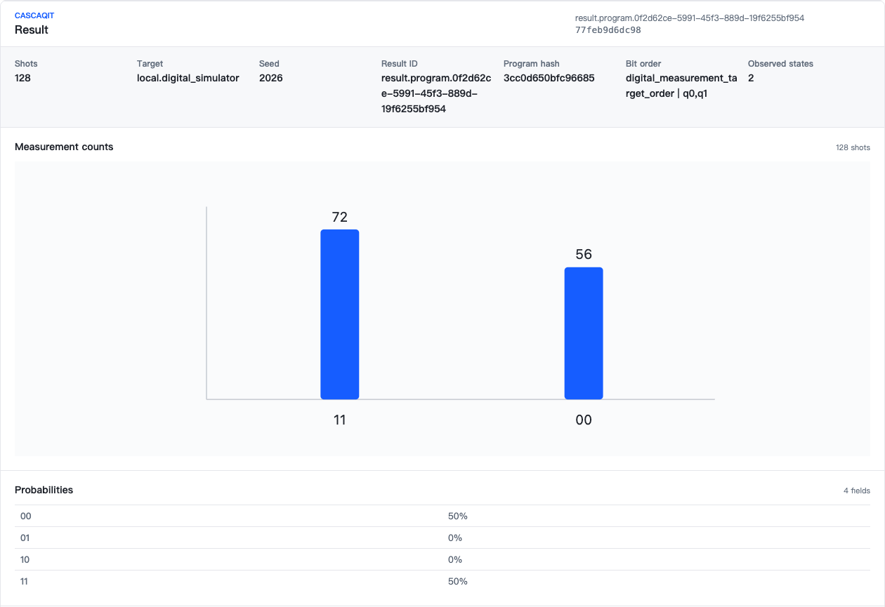
One actual run of the Bell template: 56 counts for 00 and 72 for 11. Compare probabilities and total shots; your counts need not match this capture. The image shows the counts and probabilities portion of the result card. Open full-size image
Save the result as files
import json
from datetime import datetime, timezone
from pathlib import Path
from cascaqit import visualize

run_dir = Path("experiments") / datetime.now(timezone.utc).strftime("bell-%Y%m%dT%H%M%S%fZ")
run_dir.mkdir(parents=True, exist_ok=False)
(run_dir / "result.json").write_text(
    json.dumps(result.to_dict(), ensure_ascii=False, indent=2), encoding="utf-8"
)
(run_dir / "environment.json").write_text(
    json.dumps({name: version(name) for name in ("cascaqit", "cascaqit-jupyter", "bokeh")}, indent=2),
    encoding="utf-8",
)
visualize(result, program=circuit, output=run_dir / "report.html")
print(run_dir)
Find the printed directory in the file browser and download report.html, result.json and environment.json. Open the report in a browser on your computer. Save the notebook too, including its source and cell outputs. Report language depends on the installed SDK; changing this site's language does not change kernel output.
Try copying the notebook and removing cx(0, 1). Predict the outcomes before running it, and update the assertion that checks for 00/11 to match the new experiment. Read the result's bit-order metadata before interpreting its two-bit strings.
Next, build the same circuit in the Digital editor, or study finite-shot sampling.